Motivation

So far, we’ve simulated featureless, undulating orange grids, which I find boring. What’s really cool would be an animation of a droplet of water falling into a water surface, including all the splashing effects, like this:

A quick search tells me that this is typically done with the Volume of Fluids method — roughly, modeling voxels that are filled with fluids to different degrees. My first concern was “doesn’t that completely ignore surface tension?”, but apparently there are approaches to compensate for this (see e.g. here).

To get to this result, the first thing we need is to have a 3D grid, instead of a 2D one; or even better, have a template class that can represent any number of dimensions. This is done in commit 0c5a35a. Then we’ll have to rewrite the GLFW code to display not a 2D grid, but a 3D grid. This is very far from trivial. This post is about how we can do it with the Marching Cubes algorithm.

Marching Cubes

Marching Cubes [^2] is an algorithm from computer graphics that, given a scalar field on a rectangular grid, computes a mesh of triangles that approximates an iso-surface. Without loss of generality, we assume that we want to compute the isosurface of all points where the scalar field is zero.

The idea is to look at the spaces between the points of the grid; these spaces form cubes, with 8 mesh points forming the vertices. If the vertices do not all have the same signs, then the iso-surface passes inside the cube (because the iso-surface must separate the positive points from the positive ones. Depending on which vertices have which sign, we select a different pattern of triangles.

Algorithm

The original marching cubes [^2] had 14 cases. However, it did not take into account ambiguities, which could cause it to generate holes in the surface [^1]. The updated MC algorithm that we are using goes as follows:

1. For a given combination of “on” and “off” vertices, find which of the 14 cases applies.

2. The case may have multiple sub-cases; we need to run some face tests and/or the interior test to decide which sub-case applies.

Cases

There are 2^8 = 256 combinations of “on” and “off” vertices; we reduce them to 14 cases by exploiting rotations (a cube has 23 possible rotations plus the “identity” rotation), and the fact that the “on” and “off” vertices can be swapped (the surface then still separates “on” from “off” vertices - the surface normal has to be inverted though). We do not exploit symmetry; the only case where that would play a role (in other words, the only case that is chiral) is case 11, which we are happy to duplicate into its chiral opposite, case 14.

Tests

When a face has two diagonally opposed corners to one side of the isosurface, and the two other corners to the other side, the face test tells you whether the positive corners or the negative corners are connected, like this:

Similarly, when two diagonally opposed vertices of the cube have the same sign, and there are some vertices with a different sign in between, the center test tells you whether the two vertices are connected or not:

Both tests operate under the assumption that the function varies trilinearly inside the cube.

Based on the test results, we then select a sub-case. For example in the two plots above, the positive-negative pattern (0 and 7 positive, the rest negative) tells us that we are in case 4; depending on the result of the center test, we have to select either subcase 4.1 (points not connected) or case 4.2 (points connected).

Symmetry

The cases are given up to symmetry, i.e. the combination (vertices 1 and 6 positive, the rest negative) should be turned into (0 and 7 positive, the rest negative), which we recognize as corresponding to case 4. Additionally, the sub-cases are also given up to symmetry.

We’ll distinguish between “original” coordinates, which is how the cube actually is, and the “canonical” coordinates, which is how the current case or subcase is given in the literature. In the example above, (1,6) are the original coordinates of the positive vertices; then we turn the cube to map them into (0,7), which are the canonical positive vertices of case 4. Let’s take the most complicated case, case 13.

We first have to recognize the pattern of positive edges, and turn the cube so that it corresponds to the canonical case 13. Then, we perform 6 face tests and one interior test. If there are more negative face tests than positive ones, we negate the value of each vertex (this also negates the values of the face tests) and rotate the cube to be in the canonical case 13 again, but now with more positive than negative tests.

If none of the tests are positive, we are in case 13.1. If one of them is positive, case 13.2 — but it has to be rotated to match which face is positive. For two positives, we assume that the two positives are on adjacent faces and rotate case 13.3 to fit. (Why are we allowed to assume that the positive faces are adjacent? Because the assumption of tri-linearity means that if there were two positives on opposite faces, then all faces would be positive, not only these two.)

What to precompute

We have to decide on a trade-off: what do we precompute and what do we compute at runtime? In other words, where do we use lookup tables and where do we use if-statements? One extreme would be to build a lookup table of 256 × 2^7 (the number of possible test results) entries, where each cell is a list of triangles. The other extreme would be, whenever we encounter a bit-pattern, to try all rotations of it and see whether it matches any canonical case.

My compromise is the following:

• There is a lookup table that maps positive/negative vertex patterns to a rotation + a case (1-14).

• We already compute the points where the isosurface intersects the edge (there are 12 edges, but not all of them are crossed by the isosurface). At this point, we have every geometrical information about the cube available as an array. This means that rotations can be implemented as permutations (of both the vertices and edges).

• The CPU performs the rotation, then looks up the number of tests for the case and performs all these tests (on the rotated cube).

• There is a per-case lookup table that maps test results to a rotation + a subcase.

• The CPU performs the rotation again, then draws triangles between the points computed in step 2. We computed the 3D points back when the cube was in “original” coordinates, but the array containing them has been permuted to correspond to the “canonical” list of 3D points for this case. So we can just construct triangles from those points in the order in which they are given, without having to permute things back.

How to generate cases

To describe the triangle patterns for each case, I used Python. The data was then translated to C by introspecting the Python data structures, and writing them to a C header; then writing the data as a .c file. The files are then compiled as usual by the compiler.

A nice thing is that I now also have the data structures available in Python. Translating the algorithm from C++ to Python is trivial, which allows me to plot Marching Cubes in Python, and in particular to get an interactive visualization of different cube patterns.

To showcase this, I’ve uploaded the visualization publicly: https://warggr.github.io/waves-on-cuda/scripts/marching_cubes/html/. Thanks to Pyodide, it is possible to run Python (including Matplotlib and a lot of other third-party modules) in the browser as a static webpage, without needing a server.

Other implementations

How does my implementation compare to others?

I added two other Marching Cubes implementations into my CMake project, writing a tiny wrapper so that they are replacements for my marching_cubes function.

• I could not find the source code for the original implementation of Marching Cubes 33 by Lewiner et al. [^3] (they provide a link that is now dead.)

• The first implementation is from Custodio et al., based on their 2013 paper [^4]. They fix three issues in the MC33 algorithm.

• The second implementation is from Vega et al., the authors of [^1], which was published in 2019. They state that the main contribution of their paper is the correct execution of the interior test, and the efficiency of their implementation.

Comparison

Both implementations are much more efficient than mine:

Implementation	Runtime [ms]
Mine	173
Custodio et al.	59
Vega et al.	54

I noticed that both implementations return early when all vertices have the same sign — this is the most common case, so this makes a big difference. After adding an early-return to my code, the runtime decreased to 100ms.

A likely cause for the slowness of my implementation is that I tried to separate the algorithm from the data; each case is processed the same, but based on the case-specific data in the lookup table. The code from the literature (e.g. L. Custodio’s code here) is longer and more branch-heavy. My code was easier (and less boring) to write, but this has a cost in terms of speed.

Future steps

First, there are still some bugs in my implementation. For example, I always compute the face test between the bottom-left and top-right vertex of a face, no matter how the cube is rotated; this is of course incorrect.

Second, it might be possible to implement Marching Cubes on the GPU, using a compute shader and/or a geometry shader. This might make the program faster.

Finally, there are many ways how the Marching Cubes implementation could be sped up. For example, we currently save different sub-cases as lists of triangles, where each triangle is saved as a list of vertices. But the vertices of the triangles are the same for each sub-case of the same case. Maybe vertices could be saved for a case, and then each sub-case could only contain indices indicating how these vertices are connected.

Conclusion

The code is now able to visualize 3D grids thanks to a Marching Cubes implementation. Despite the apparent simplicity of Marching Cubes, there are many details to pay attention to. Open-source implementations are much faster and so should be preferred.

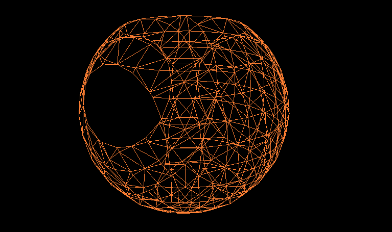
Cover image: a sphere plotted with Marching Cubes, more precisely a visualization of the field

$$(x - 5)^2 + (y-5)^2 + (z-5)^2$$

I don’t know why three sides are cut off; I probably made an off-by-one error somewhere.

References

[^1]: Vega, D., Abache, J., & Coll, D. (2019). A fast and memory-saving marching cubes 33 implementation with the correct interior test. In Journal of Computer Graphics Techniques 8.3.

[^2]: Lorensen, W. E., & Cline, H. E. (1998). Marching cubes: A high resolution 3D surface construction algorithm. In Seminal graphics: pioneering efforts that shaped the field (pp. 347-353).

[^3] Lewiner, T., Lopes, H., Vieira, A. W., & Tavares, G. (2003). Efficient Implementation of Marching Cubes’ Cases with Topological Guarantees. Journal of Graphics Tools, 8(2), 1–15. https://doi.org/10.1080/10867651.2003.10487582

[^4] Custodio, L., Etiene, T., Pesco, S., & Silva, C. (2013). Practical considerations on Marching Cubes 33 topological correctness. Comput. Graph. 37, 7 (November, 2013), 840–850. https://doi.org/10.1016/j.cag.2013.04.004