Part 5: The Volume of Fluid method
In this post, I'll walk through my implementation of the Volume of Fluid method. The overall motivation is to simulate 3D waves and droplets of water, like this:

In practice, this post will mostly describe "why are the incompressible Euler equations useful and how can we simulate them?"
Models
There is one reality, and there are different models of it. Some models include:
the Navier-Stokes equations (our most complete understanding of fluid dynamics, except for more advanced models that involve atomic theory; very difficult to solve)
the Euler equations (a simplified model where we neglect friction and heat transfer)
the incompressible Euler equations (a simplified model that neglects fluid compression)
a computer simulation of the incompressible Euler equations (an inaccurate model, because it can only represent discrete timesteps and machine-precision
doublevalues instead of real numbers)my implementation of the simulation of the incompressible Euler equations (which might introduce some bugs)
Another model of reality is of course "intuition", i.e. whatever you're doing when you're looking at a picture of a wave and thinking "that's how the wave will move in the next second".
For all of those models to be useful, they have to agree, i.e. predict the same things (at least to some extent).
The dam break
Imagine a wall of water: one meter of water to the right, and nothing to the left. (You can imagine a dam separating the water that suddenly disappeared at t=0). What do the different models tell us will happen?
Your mental model of the world should imagine the water evolving like this:
https://www.youtube.com/watch?v=i5bpA-f8FW0
The incompressible NS equations tell us a similar, but more detailed, story. (The math assumes that you are familiar with partial derivatives and the notation \(\text{div }\mathbf{u} =: \nabla \cdot \mathbf{u}\)).
The wall of water starts at rest, i.e. \(u = 0\), and evolves according to:
$$\begin{aligned} \frac{d \mathbf{u}}{d t} + \mathbf{u} \cdot \nabla \mathbf{u} &= \mathbf{f} - \frac{\nabla p}{\rho} \ \nabla \cdot \mathbf{u} &= 0 \end{aligned}$$
where
\(\mathbf{u} \in \mathbb{R}^3\) is the fluid velocity
\(p \in \mathbb{R}\) is the pressure
\(\rho \in \mathbb{R}\) is the density
\(\mathbf{f} \in \mathbb{R}^3\) are the external forces
Nonzero gravity (\(\mathbf{f} = -9.81 \rho \vec{z}\) ), and zero convective transport in the absence of velocity ( \(\mathbf{u} \cdot \nabla \mathbf{u} = 0\)), would cause a downwards velocity everywhere, if there wasn't the pressure term to balance it out.
The pressure corresponds to hydrostatic pressure, i.e. high pressure at the bottom and a low pressure at the top. This pressure exactly compensates the effect from gravity, so that the downwards velocity is zero everywhere.
But pressure is non-directed - so the high pressure at the bottom, or rather the difference between this high pressure and the low air pressure next to it, will cause the fluid to move to the right at the bottom. Similarly, the fluid will move to the left at the top.
Now that fluid is leaking at the bottom, the fluid at the top will also move downwards due to gravity.
The whole wall of water will spectacularly break down.
Here, we have an agreement between intuition, the above video, and the incompressible Navier-Stokes equations. So all of these models are useful!
Solving the incompressible Euler equations
The incompressible Euler equations are already a simplified model, but they are still differential equations involving continuous quantities over continuous space evolving in continuous time. To simulate them, we need to discretize them both in time and in space (casting them from a differential equation to a difference equation) and then to solve them.
The incompressible Euler equations are as follows (from Wikipedia):
$$\begin{align} \frac{\partial \rho}{\partial t} + \mathbf{u} \cdot \nabla\rho &= 0 & \text{(a)} \ \frac{\partial \mathbf{u}}{\partial t} + \mathbf{u} \cdot \nabla \mathbf{u} &= - \frac{\nabla p}{\rho} + \mathbf{f} & \text{(b)} \ \nabla \cdot \mathbf{u} &= 0 & \text{(c)} \end{align}$$
In our case, we also have a no-slip boundary condition at the walls: \( \vec{n} \cdot \mathbf{u} |_{\partial \Omega} = 0\).
(a) represents the mass conservation, (b) the impulse conservation, and (c) the incompressibility. (a) is handled by VoF, because VoF is what we use to model mass and density. We will (somewhat arbitrarily) first solve (b) and (c) for the velocity \(\mathbf{u}\), then solve (a) based on that velocity.
(Reference for the previous paragraph: https://web.stanford.edu/class/me469b/handouts/incompressible.pdf)
The projection method
When trying to solve (b), we encounter the problem that $p$ has no explicit expression, and isn't even conserved between time steps. The solution is to use a projection method. The idea is to solve (b) and (c) at the same time and solve them for both \(\mathbf{u}\) and $p$.
This section is based on https://orbi.uliege.be/bitstream/2268/2649/1/BBEC9106.pdf.
The idea behind the projection method was described above: we consider "what would the velocity do if there was no pressure?", i.e. we first compute a "transport velocity" \(\mathbf{u}_\text{trans}\) that solves the first equation without the pressure term. Then we compute what the pressure must be to fulfill both (ii) and (iii).
We partly discretize the equations with an explicit scheme into
$$\begin{align} \frac{\mathbf{u}^{(i+1)} - \mathbf{u}^{(i)}}{\Delta t} + \mathbf{u}^{(i)} \cdot \nabla \mathbf{u}^{(i)} &= - \frac{\nabla p}{\rho} + \mathbf{f} \ \nabla \cdot \mathbf{u}^{(i+1)} &= 0 \end{align}$$
$$\implies \begin{align} \mathbf{u}^{(i+1)} &= \mathbf{u}^{(i)} - \Delta t ( \mathbf{u}^{(i)} \cdot \nabla \mathbf{u}^{(i)} ) - \Delta t \frac{\nabla p}{\rho} + \Delta t \mathbf{f} \ \nabla \cdot \mathbf{u}^{(i+1)} &= 0 \end{align}$$
Define \(\mathbf{u}_\text{trans} := -\mathbf{u}^{(i)} \cdot \nabla \mathbf{u}^{(i)} + \mathbf{f}\)
$$\begin{align} \mathbf{u}^{(i+1)} &= \mathbf{u}^{(i)} + \Delta t \mathbf{u}_ \text{trans} - \Delta t \frac{\nabla p}{\rho} \ \nabla \cdot \mathbf{u}^{(i+1)} &= \nabla \cdot \mathbf{u}^{(i)} = 0 \ \implies \nabla \cdot (\mathbf{u}\text{trans} -\frac{\nabla p}{\rho}) &= 0 \ \implies \nabla \cdot \frac{\nabla p}{\rho} &= \nabla \cdot \mathbf{u}\text{trans} \end{align}$$
where we can compute the right-hand side with finite differences. Then we can solve this differential equation and get $p$ (up to a constant; we can arbitrarily set the mean pressure to 0).
You might wonder why we solve for $p$ while we're only interested in \(\frac{\nabla p}{\rho}\). But the equation \(\frac{\nabla p}{\rho} = \mathbf{u}_\text{trans}\) does not have a unique solution for \(\nabla p\); rather, it must be combined with the knowledge that \(\nabla p\) is a gradient (and therefore rotation-free) to get a unique solution. This is what the Poisson-like equation is trying to achieve.
Algorithm:
$$\begin{aligned} \mathbf{u}\text{trans} &\leftarrow -( \mathbf{u}^{(i)} \cdot \nabla \mathbf{u}^{(i)} ) + \mathbf{f} \ p &\leftarrow solve\left(\nabla \cdot \frac{\nabla p}{\rho} = \nabla \cdot \mathbf{u}\text{trans}\right) \ \mathbf{u}^{(i+1)} &\leftarrow \mathbf{u}^{(i)} + \Delta t \mathbf{u}_\text{trans} - \Delta t \frac{\nabla p}{\rho} \end{aligned}$$
To compute \(\mathbf{u}_\text{trans}\): Use the fact that (using index notation):
$$\mathbf{u} \cdot \nabla \mathbf{u} = u_i \frac{\partial u_j}{\partial x_i} = \frac{\partial u_i}{\partial x_i} u_j + u_i \frac{\partial u_j}{\partial x_i} = \frac{\partial u_i u_j}{\partial x_i} = \nabla \cdot (\mathbf{u} \otimes \mathbf{u})$$
because \(\frac{\partial u_i}{\partial x_i} = \nabla \cdot \mathbf{u} = 0\). So we can compute \(\mathbf{u} \cdot \nabla \mathbf{u}\) by computing \(\mathbf{u} \otimes \mathbf{u}\) for all points and taking derivatives (or finite differences).
To compute $p$: We approximate the differential equations with finite differences. If the density was constant, this would be a Poisson equation; but the density is not constant, so we need a slightly different stencil: (here \(p_i\) denotes "$p$ at cell $i$".)
$$\nabla \cdot \frac{\nabla p}{\rho} \approx \frac{1}{\Delta x^2} (1/\rho_{i+1/2} (p_{i+1} - p_{i}) - 1/\rho_{i-1/2} (p_{i} - p_{i-1}))$$
This corresponds to the stencil
$$\frac{1}{\Delta x^2} \begin{bmatrix} \frac{1}{\rho_{i+1/2}} & (-\frac{1}{\rho_{i+1/2}} - \frac{1}{\rho_{i-1/2}}) & \frac{1}{\rho_{i-1/2}} \end{bmatrix}$$
We then solve this system of finite difference equations with Eigen's Conjugate Gradient solver, which is recommended for the 3D Poisson equation.
Discretization in space: I discretize
the pressure on the cell centers; therefore the pressure gradient on the cell faces can be approximated trivially by the pressure difference
\(\rho\) is also given on the cell centers, therefore the \(\rho_{i \pm 1/2}\) above require averaging
\(\mathbf{u}\) on the cell faces. therefore \(\nabla \cdot \mathbf{u}\) can be approximated trivially on the cell centers
\(\mathbf{u} \otimes \mathbf{u}\) on the cell centers by averaging the velocities from the neighboring faces
\(\mathbf{u}_\text{trans}\) on the cell centers; it involves \(\mathbf{f}\), given on the cell centers, and \(\mathbf{u} \otimes \mathbf{u}\)
I think this is the discretization that requires the least effort.
Volume of Fluid and solving the density equation
This section is adapted from Volume of Fluid: A Brief Review.
Volume of Fluid (VoF) tracks the distribution of two fluids in a system. Since the fluids have different, but constant, densities, tracking fluid distributions is equivalent to enforcing the mass conservation from the Navier-Stokes equations:
$$\frac{\partial \rho}{\partial t} + \mathbf{u} \cdot \nabla\rho= 0$$
We specifically use the geometric VoF approach, as opposed to the algebraic VoF approach; geometric VoF is more standard. In geometric VoF, we reconstruct the fluid surface to decide how the fluid evolves.
To reconstruct the fluid interface, we use the piecewise linear interface calculation (PLIC) approach. We look at a 3x3x3 cube of cells and their volume fractions, find the normal vector that best matches the volume fractions in those cells, and set the center cell's normal vector as that vector.
Once we have the normal vector and the volume fraction in a cell, we can compute the "cell wet wall sizes", i.e. the fraction of a the cell wall sizes that is occupied by the fluid. The following image shows in blue the cell wet wall sizes in a given configuration:

Then, we compute the flux between cells by multiplying the velocity with the cell wet wall size. We should also take into account the fact that these walls have a slope. In 2D, the following figure explains the slope (figure adapted from Volume of Fluid Method: a Brief Review):

The wet wall size is the blue line on the right; the advected volume is not just the rectangle given by \(\text{wallsize} \cdot u_{i+\frac{1}{2},j} \Delta t\), but rather the trapeze highlighted in blue. A special case happens if the time step is large enough that the blue trapeze meets the top line. In 3D, this is even more complicated. So I just ignored the slope and considered only the rectangle.
Then, we advect the volumes and update the volume fraction of each cell. Note that there is no guarantee that the volume fractions after the advection are still in the interval $[0, 1]$. If we were using an advanced VoF scheme, we'd have such guarantees. But instead we just clamp them to $[0, 1]$ and do not worry too much about the volume loss.
Various fun implementation details
I added Python bindings for the wet-wall-size formula, so that I can unit-test it from Python. This also allows me to visualize wet wall sizes, which is how I generated the plot above.
I added Numpy loading of matrices, instead of hardcoding the initial conditions. For this, I used the cnpy library.
Results
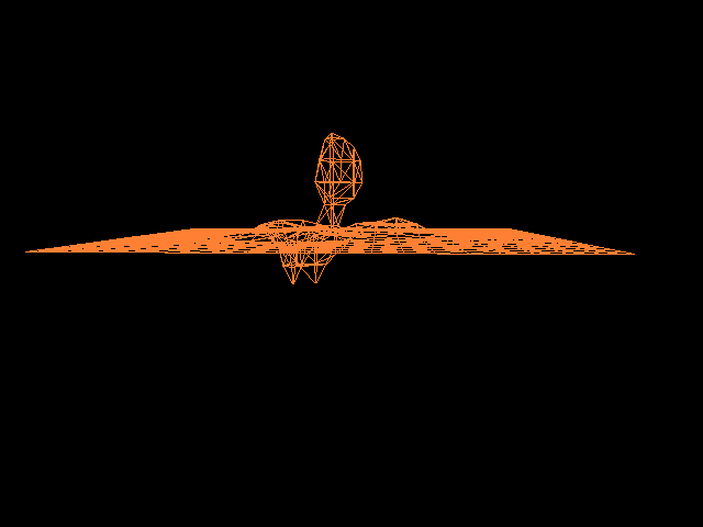
The simulation results for a dambreak-like scenario look like this:

The overall shape of the dambreak is as it should, but there is still some non-physical behavior with non-fluid bubbles forming behind the wave. There is another error (possibly linked) where the mesh becomes completely chaotic at the end (the program then usually ends with a failed assertion because some values are NaN).
The main computational bottleneck is the Eigen matrix solver to get the pressure. As far as I know, this is a fundamental limitation of the incompressible Euler equations. In the incompressible mode, the pressure everywhere is coupled and any grid point can influence any other grid point (this is different from the compressible Euler equations, which have only conservation equations and where there is a "finite signal speed").
Conclusion and future steps
This post outlined the implementation of a volume-of-fluid (VoF) scheme to simulate the incompressible Euler equations. The behavior of the simulation code mostly follows physics, but still has a few issues. The remaining steps are:
Fix any remaining VoF bugs
Use a more advanced VoF method with volume conservation guarantees
Implement the compressible Euler equations
Porting the solver to CUDA